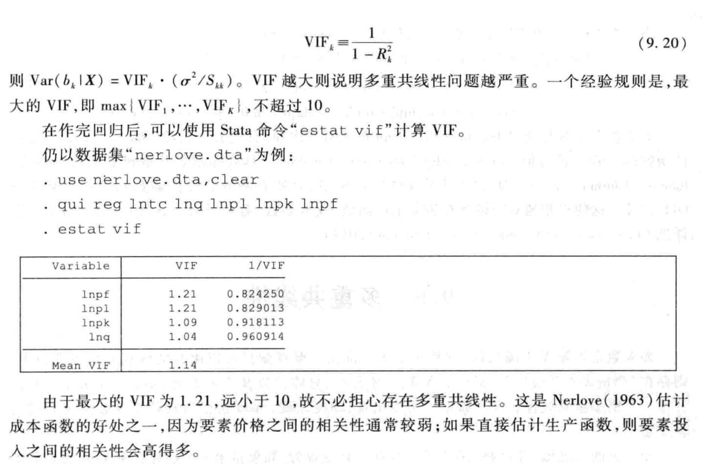
** 考察年龄、教育程度、婚姻和12岁以下孩子数量之间的相关性 corr age education married children
** 考察年龄、教育程度、婚姻和12岁以下孩子数量之间的多重共线性 collin age education married children
********************* 结果展示 ********************* // 相关性 · corr age education married children | age educat~n married children -------------+------------------------------------ age | 1.0000 education | 0.2377 1.0000 married | 0.3459 0.2768 1.0000 children | 0.0343 -0.0344 -0.1052 1.0000
// 多重共线性 · collin age education married children Collinearity Diagnostics
SQRT R- Variable VIFVIF Tolerance Squared ---------------------------------------------------- age 1.17 1.08 0.8533 0.1467 education 1.11 1.05 0.9002 0.0998 married 1.21 1.10 0.8285 0.1715 children 1.02 1.01 0.9830 0.0170 ---------------------------------------------------- MeanVIF 1.13
Cond Eigenval Index --------------------------------- 1 4.3149 1.0000 2 0.4305 3.1659 3 0.1966 4.6848 4 0.0382 10.6266 5 0.0197 14.7850 --------------------------------- Condition Number 14.7850 Eigenvalues & Cond Index computed from scaled raw sscp (w/ intercept) Det(correlation matrix) 0.7792

 alipay