陈强等(2025)《双重差分法的安慰剂检验:一个实践的指南》一文系统梳理了标准 DID、交叠 DID、连续 DID、队列 DID 等多种差分法的安慰剂检验思路和方法,并提供了标准 DID 和交叠 DID 的安慰剂检验程序。本文对将对其提供的安慰剂检验程序进行梳理和复现,推荐大家先阅读原论文,再结合推文附件中的代码进行复现。
HDFE Linear regression Number of obs = 140,432 Absorbing 2 HDFE groups F( 1, 535) = 5.23 Statistics robust to heteroskedasticity Prob > F = 0.0226 R-squared = 0.0308 Adj R-squared = 0.0253 Within R-sq. = 0.0002 Number of clusters (county) = 536 Root MSE = 0.3848
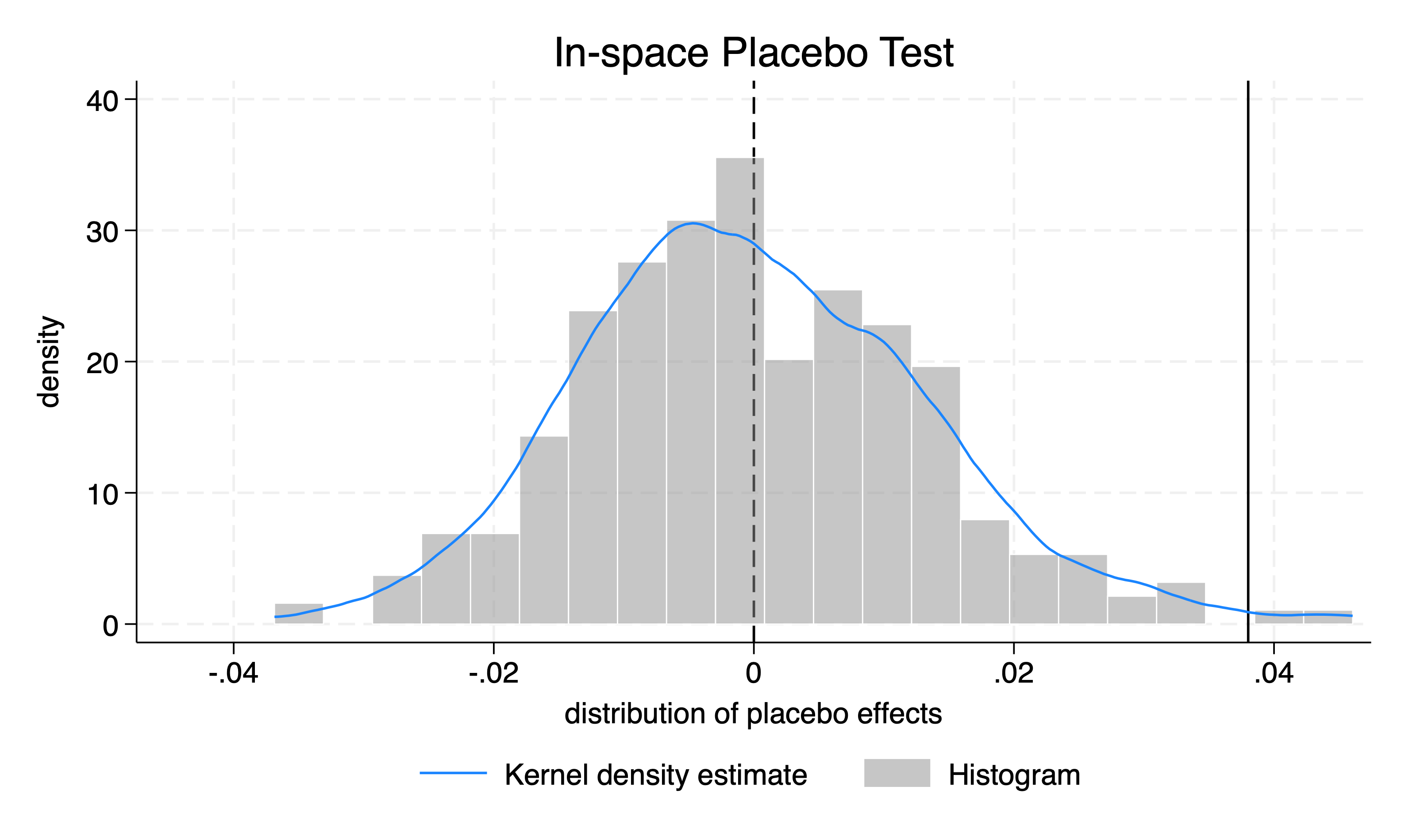
Implementing in-space placebo test using fake treatment units: Simulations (500):.........10.........20.........30.........40.........50.........60.........70.........80.........90.........100...... > ...110.........120.........130.........140.........150.........160.........170.........180.........190.........200.........210....... > ..220.........230.........240.........250.........260.........270.........280.........290.........300.........310.........320........ > .330.........340.........350.........360.........370.........380.........390.........400.........410.........420.........430......... > 440.........450.........460.........470.........480.........490.........500 Results of in-space placebo test results using fake treatment units: -------------------------------------------------------------- | | P-value | Coefficient | Two-sided Left-sided right-sided -----------+-------------+------------------------------------ canal_post | 0.038014 | 0.0080 0.9920 0.0080 -------------------------------------------------------------- Note: (1) The two-sided p-value is the frequency that the absolute values of the placebo effects are greater than or equal to the absolute value of estimated treatment effect. (2) The left-sided (right-sided) p-value is the frequency that the placebo effects are smaller (greater) than or equal to the estimated treatment effect.
Finished.
需要注意的是,估计结果表的重点不在于前面的估计系数0.038014 ,而是后面的 P 值。
结果表中的系数是上面使用 reghdfe 命令进行 DID 估计得到的系数。
上表中包含三个 P 值,分别是双边检验、左边检验和右边检验的 P 值。双边检验的目的是估计系数的绝对值 \(|\hat {\delta}^*|\) 是否显著区别于 0,左边检验是检验估计系数是否满足 \(\hat {\delta}^* \lt 0\),右边检验是检验估计系数是否满足 \(\hat {\delta}^* \gt 0\)。
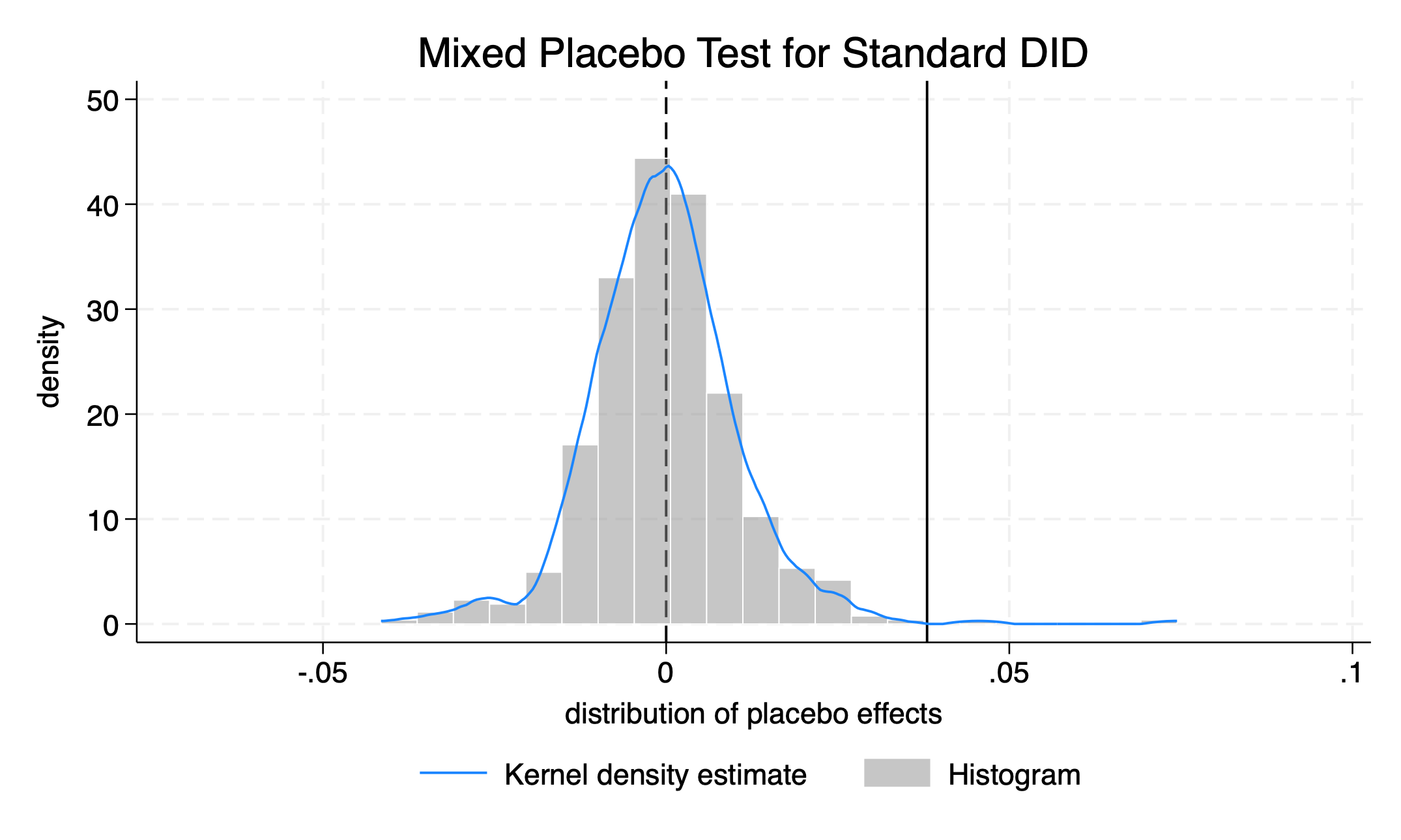
Implementing mixed placebo testfor standard DID (version 1) using both fake treatment units and times: ------------------------------------------------------------------------- The number of units randomly | The range within which fake selected as fake treatment units | treatment times are randomly selected ----------------------------------+-------------------------------------- 73 | [1651, 1911] ------------------------------------------------------------------------- Simulations (500):.........10.........20.........30.........40.........50.........60.........70.........80.........90.........100...... > ...110.........120.........130.........140.........150.........160.........170.........180.........190.........200.........210....... > ..220.........230.........240.........250.........260.........270.........280.........290.........300.........310.........320........ > .330.........340.........350.........360.........370.........380.........390.........400.........410.........420.........430......... > 440.........450.........460.........470.........480.........490.........500 Results of mixed placebo testfor standard DID (version 1) using both fake treatment units and times: -------------------------------------------------------------- | | P-value | Coefficient | Two-sided Left-sided right-sided -----------+-------------+------------------------------------ canal_post | 0.038014 | 0.0060 0.9960 0.0040 -------------------------------------------------------------- Note: (1) The two-sided p-value is the frequency that the absolute values of the placebo effects are greater than or equal to the absolute value of estimated treatment effect. (2) The left-sided (right-sided) p-value is the frequency that the placebo effects are smaller (greater) than or equal to the estimated treatment effect.
Finished.
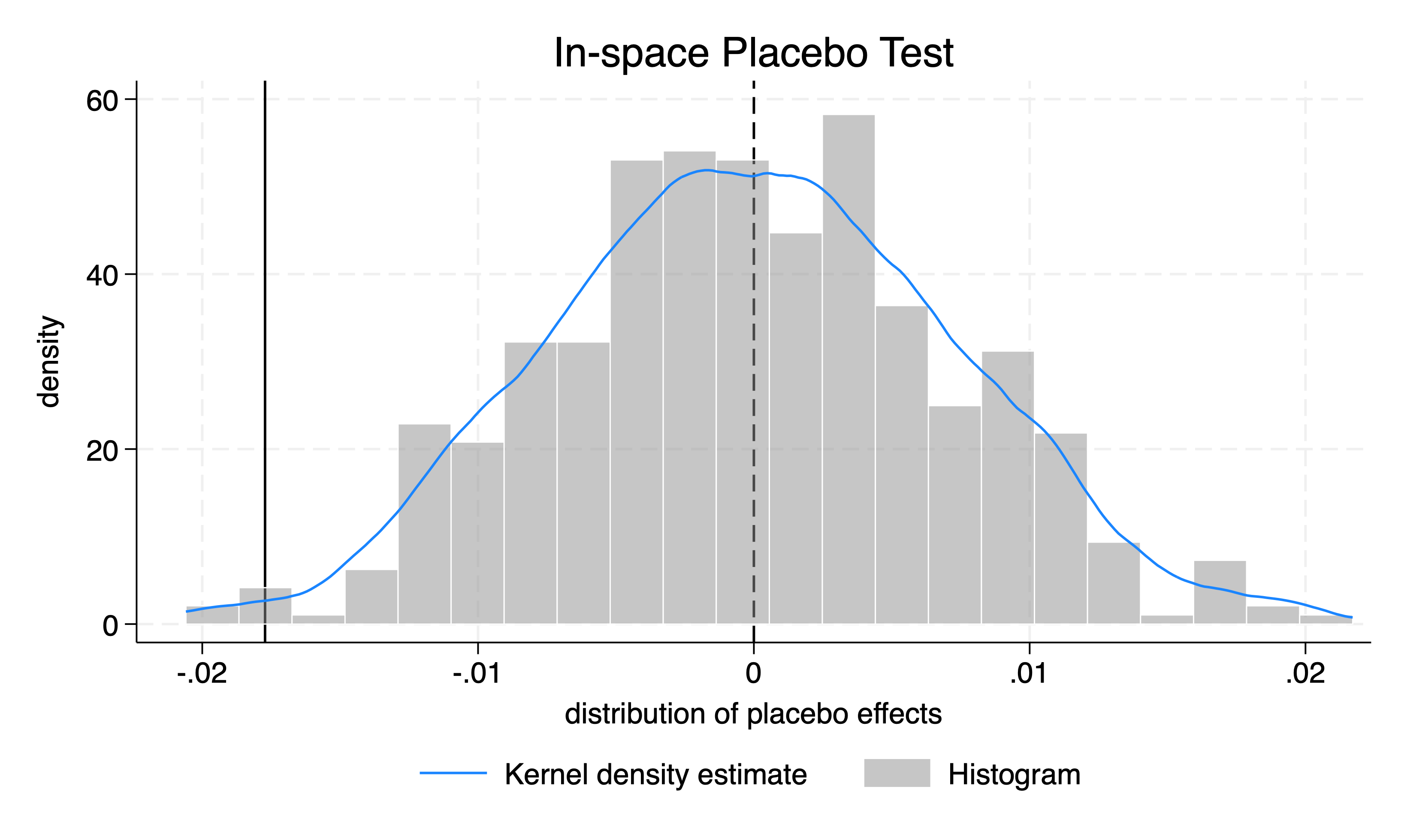
上面混合安慰剂检验结果的解读方法,和个体安慰剂检验是基本一致的。由于基准回归系数是正的,因此我们重点关注双边检验和右边检验,可以发现其 P 值均小于 0.01,在 1% 水平上通过了混合安慰剂检验,即基准回归估计的正系数是稳健的。同时我们将真实的估计系数放到密度分布图中,可以发现真实的估计系数位于右侧长尾处,再次验证基准回归结果是稳健的。
交叠 DID 的回归方程仍可采用标准形式表达,但由于每个个体的处理起始时间不同,处理变量 \(D_{it}\) 无法表示为统一的交互项 \(\text{treat}_i \times \text{post}_t\);其传统估计方法为双向固定效应(TWFE)估计量,对应的安慰剂检验也通常基于 TWFE 实施。与标准 DID 类似,交叠 DID 的安慰剂检验也可分为时间、空间、混合与外部安慰剂检验四种类型。由于标准 DID 是交叠 DID 的特例(前者只有两个组群,即处理组与控制组;而后者可有多个组群,根据受处理时间而分类),故标准 DID 的安慰剂检验也可视为交叠 DID 安慰剂检验的特例。
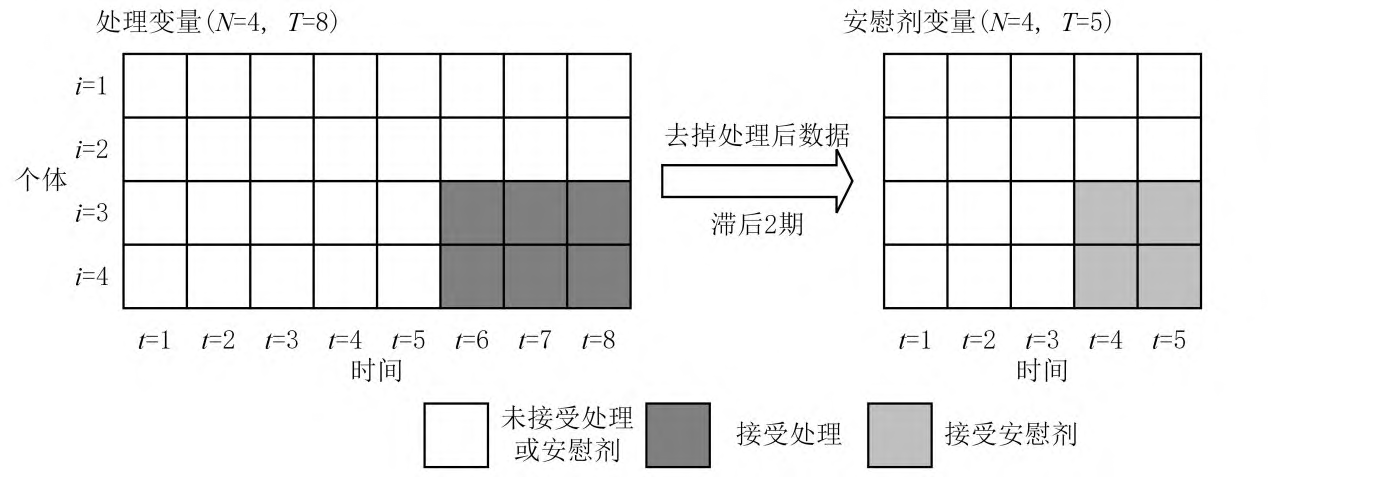
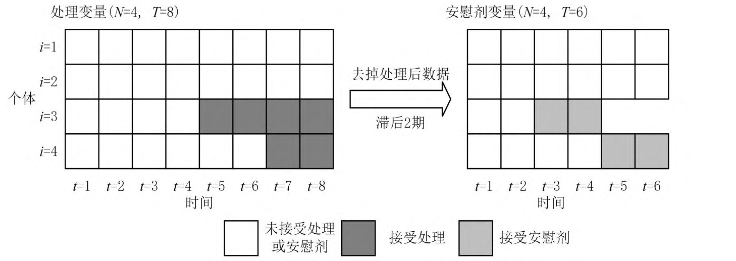
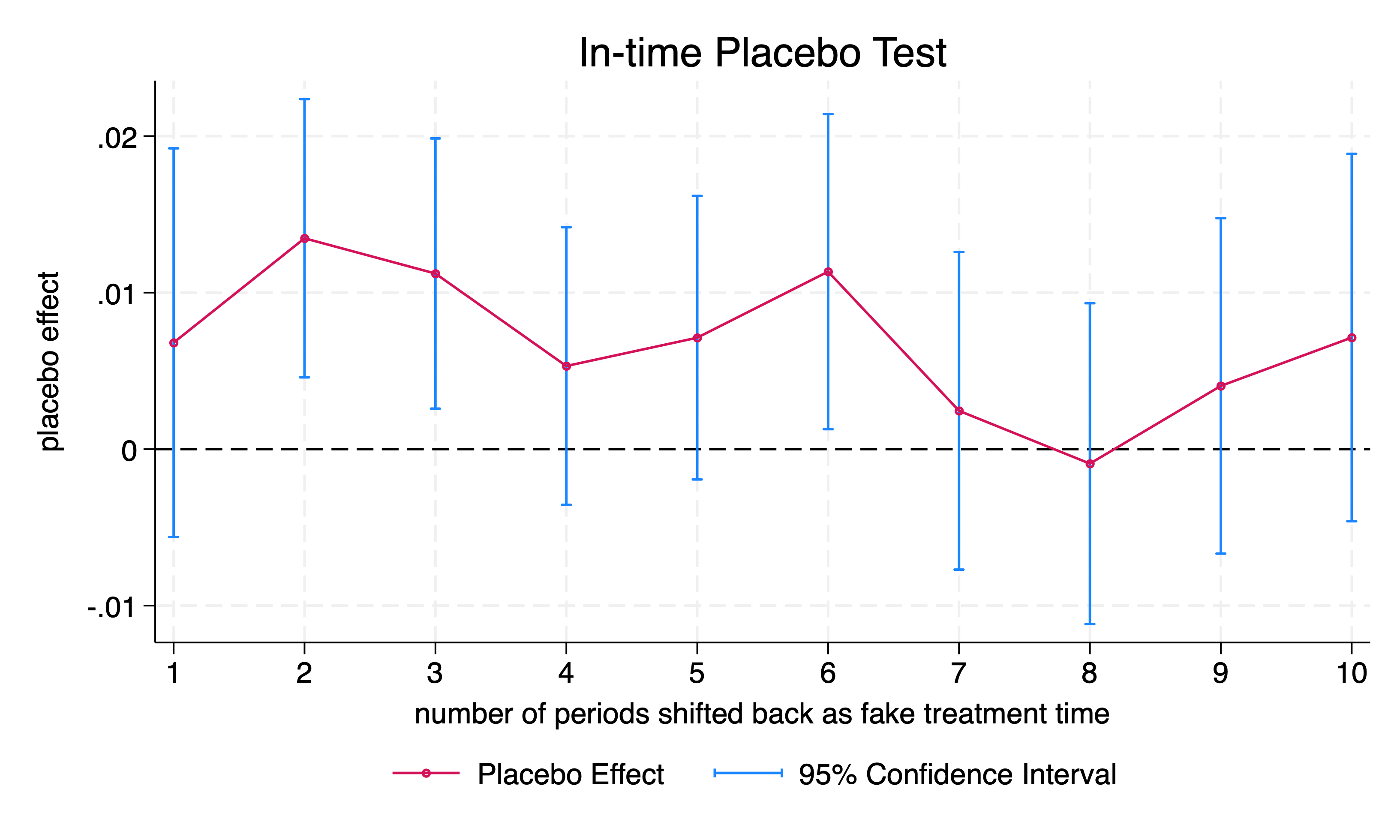
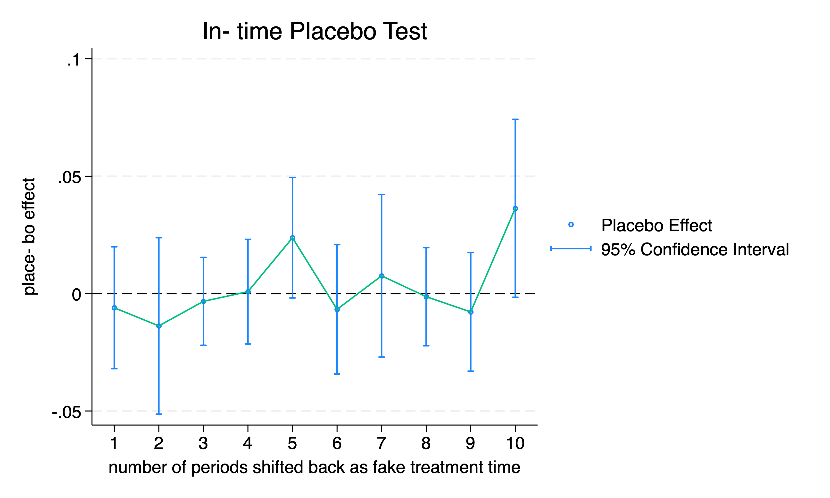
交叠 DID 的时间安慰剂检验通过滞后处理时间设定伪处理期,在剔除真实处理后观测值后进行 DID 估计,以检验在未实际受处理前是否已存在显著效应,从而识别潜在的时变混杂因素。如下图所示,删除原干预组处理后的样本(\(i=3\),\(5 \leq t\leq 8\) 和 \(i=4\),\(7 \leq t\leq 8\)),并将干预时间滞后 2 期。
1.2 交叠 DID 的个体安慰剂检验
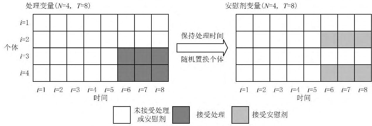
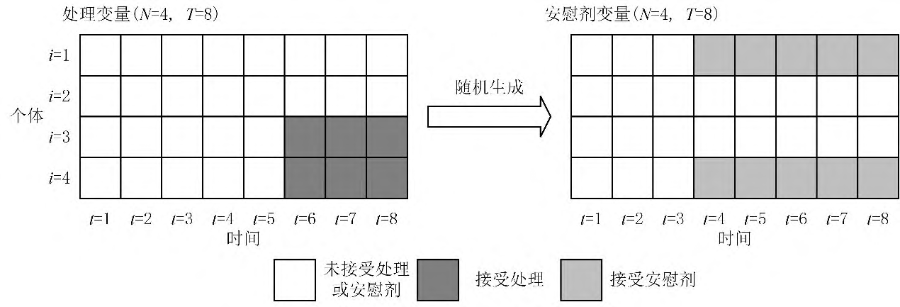
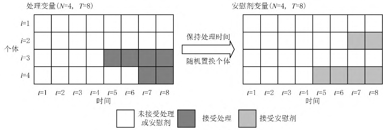
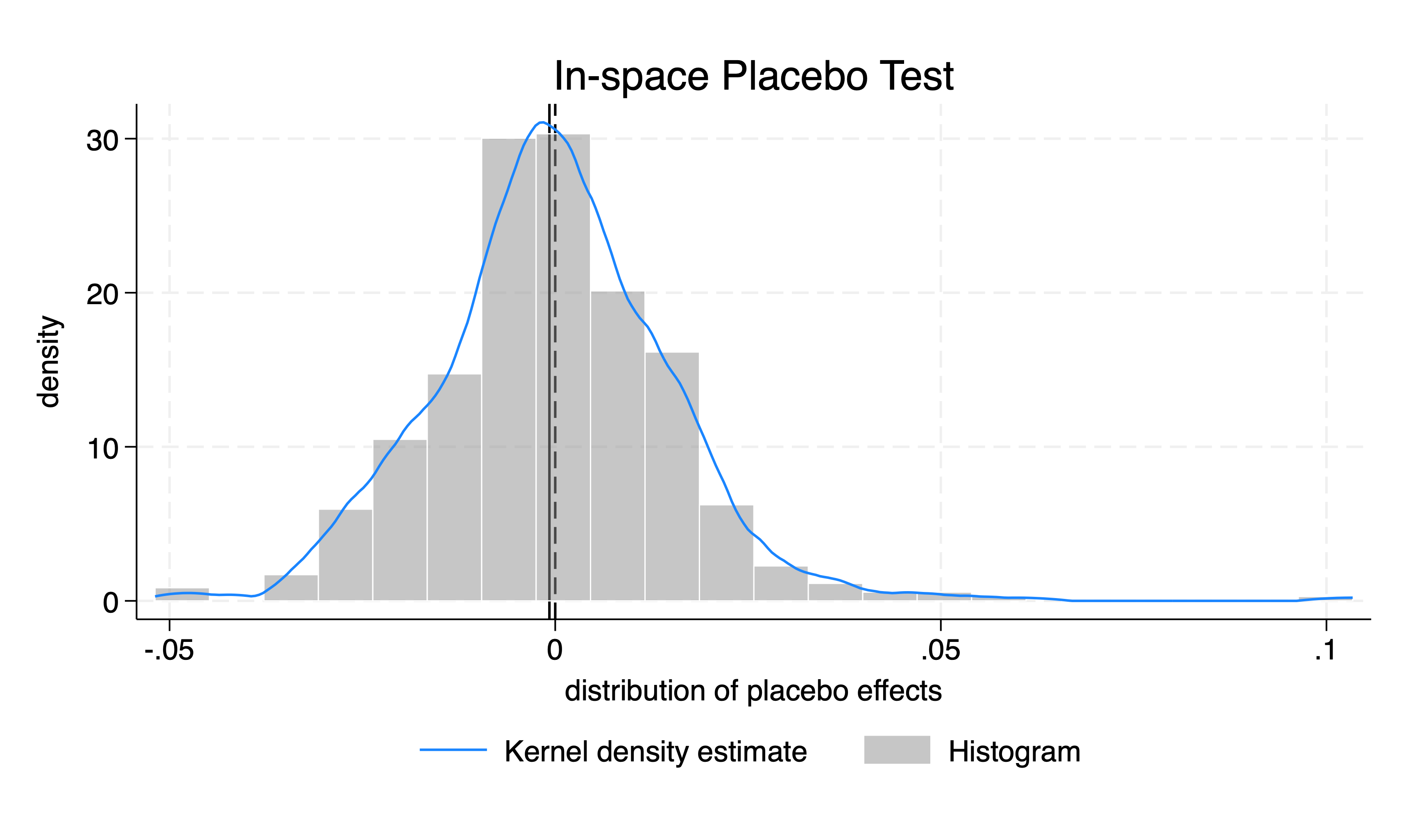
类似于标准 DID,在交叠 DID 中,也可以通过重新分配干预组和控制组,实现个体安慰剂检验。具体来看,根据样本中个体开始接受处理的不同时间,可将个体分为若干“组群”(cohorts)。交叠 DID 的空间安慰剂检验使用伪处理组,但不改变处理时间。 与标准 DID 类似,根据产生伪处理组的不同方式,交叠 DID 的空间安慰剂检验分为“非随机”与“随机”两种。下图是使用“随机”置换手段构造伪干预组,将个体 \(i=3\) 的干预行为置换到样本 \(i=4\) 上,将个体 \(i=4\) 的干预行为置换到样本 \(i=2\) 上,然后检验政策干预的效果是否仍然显著。
1.3 交叠 DID 的混合安慰剂检验
交叠 DID 的混合安慰剂检验有两种方法:一是不再保持“组群”结构,实行“无约束”的混合安慰剂检验;二是保持“组群”结构,实行“有约束”的混合安慰剂检验。
1.3.1 无约束的混合安慰剂检验
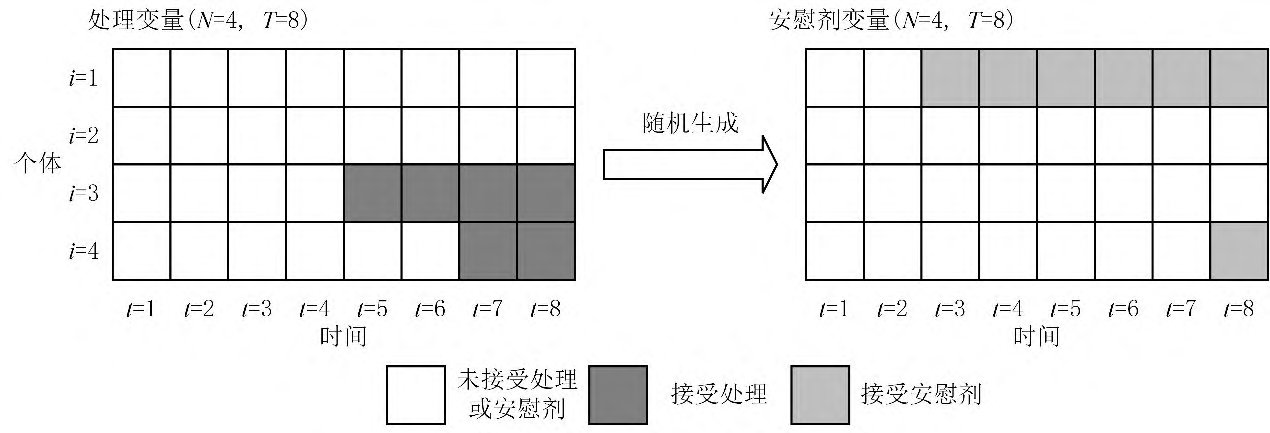
对于无约束的混合安慰剂检验,其原理是:对于样本中的每位个体,在指定范围内随机抽取一个伪干预时间 \(t^*_{i}\) 得到安慰剂样本,进行 DID 估计,并使用安慰剂效应的分布进行统计推断。
交叠 DID 个体安慰剂检验结果解读与上面标准 DID 类似,也是关注表中的 p 值、图中黑色实线的位置。基准回归的估计系数是 -0.017724,为负数,因此这里关注双边检验和左边检验的 p 值。双边检验 \(P=0.0120\),表明在 5% 水平上,估计系数的绝对值是显著区别于 0 的;左边检验 \(P=0.0060\),表明在 1% 水平上,估计系数是显著小于 0 的。同时,基于绘制的个体安慰剂检验密度分布图,可以发现真实的回归系数(黑色竖线)位于检验结果模拟分布的左侧长尾处,表明基准回归结果为负是稳健的。
Implementing in-space placebo test using fake treatment units: Simulations (500):.........10.........20.........30.........40.........50.........60.........70.........80.........90.........100.........110.........120..... > ....130.........140.........150.........160.........170.........180.........190.........200.........210.........220.........230.........240.........250..... > ....260.........270.........280.........290.........300.........310.........320.........330.........340.........350.........360.........370.........380..... > ....390.........400.........410.........420.........430.........440.........450.........460.........470.........480.........490.........500 Results of in-space placebo test results using fake treatment units: -------------------------------------------------------------- | | P-value | Coefficient | Two-sided Left-sided right-sided -----------+-------------+------------------------------------ _intra | -0.017724 | 0.0120 0.0060 0.9940 -------------------------------------------------------------- Note: (1) The two-sided p-value is the frequency that the absolute values of the placebo effects are greater than or equal to the absolute value of estimated treatment effect. (2) The left-sided (right-sided) p-value is the frequency that the placebo effects are smaller (greater) than or equal to the estimated treatment effect.
Finished.
3.3 交叠 DID 的混合安慰剂检验
3.3.1 无约束的混合安慰剂检验
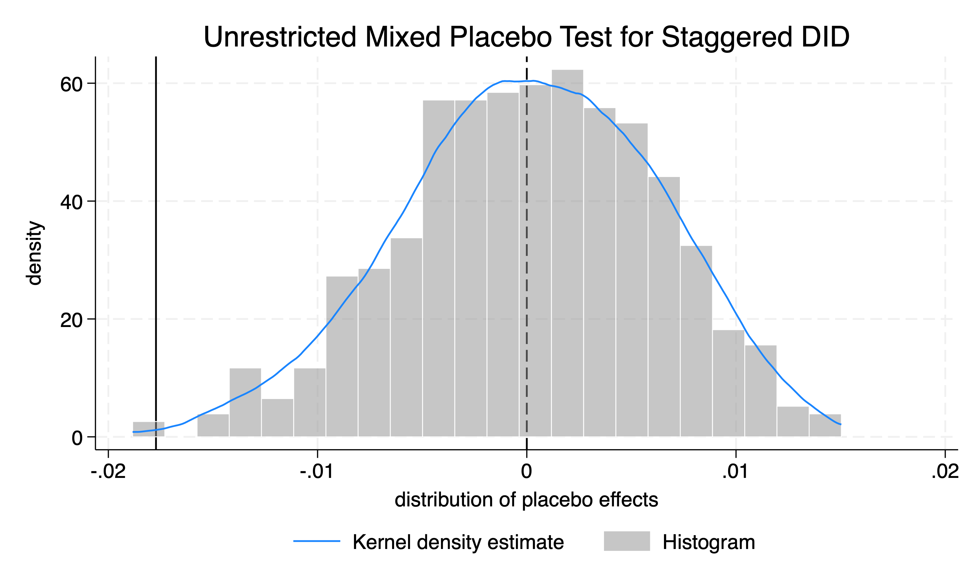
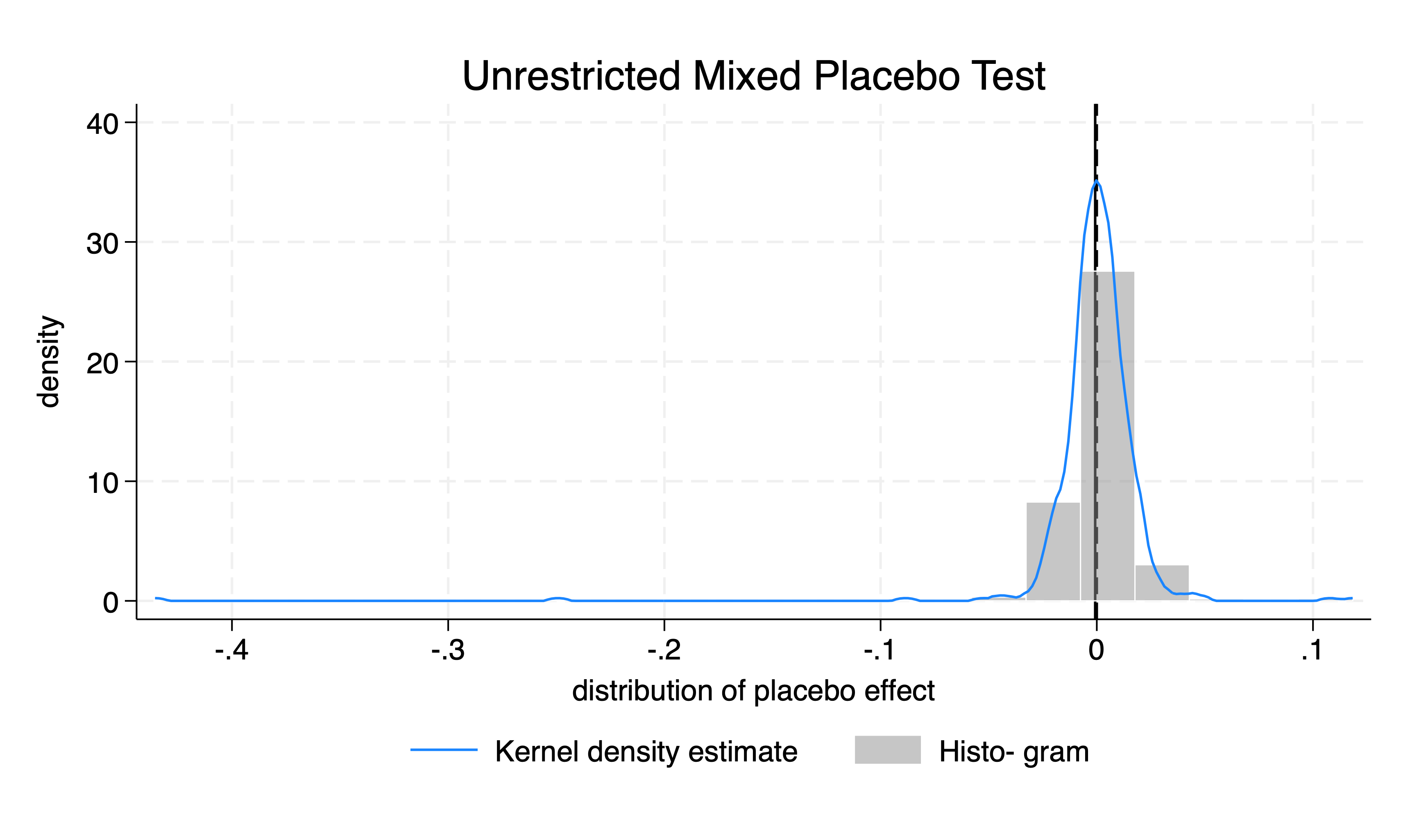
指定 pbomix(2) 以进行无约束的混合安慰剂检验,结果展示与交叠 DID 的个体安慰剂检验类似。
Implementing unrestricted mixed placebo testfor staggered DID (version 2) using both fake treatment units and times: ------------------------------------------------------------------------- The number of units randomly | Th range within which fake selected as fake treatment units | treatment times are randomly selected ----------------------------------+-------------------------------------- 49 | [1976, 2000] ------------------------------------------------------------------------- Simulations (500):.........10.........20.........30.........40.........50.........60.........70.........80.........90.........100.........110.........120..... > ....130.........140.........150.........160.........170.........180.........190.........200.........210.........220.........230.........240.........250..... > ....260.........270.........280.........290.........300.........310.........320.........330.........340.........350.........360.........370.........380..... > ....390.........400.........410.........420.........430.........440.........450.........460.........470.........480.........490.........500 Results of unrestricted mixed placebo testfor staggered DID (version 2) using both fake treatment units and times: -------------------------------------------------------------- | | P-value | Coefficient | Two-sided Left-sided right-sided -----------+-------------+------------------------------------ _intra | -0.017724 | 0.0040 0.0040 0.9960 -------------------------------------------------------------- Note: (1) The two-sided p-value is the frequency that the absolute values of the placebo effects are greater than or equal to the absolute value of estimated treatment effect. (2) The left-sided (right-sided) p-value is the frequency that the placebo effects are smaller (greater) than or equal to the estimated treatment effect.
Finished.
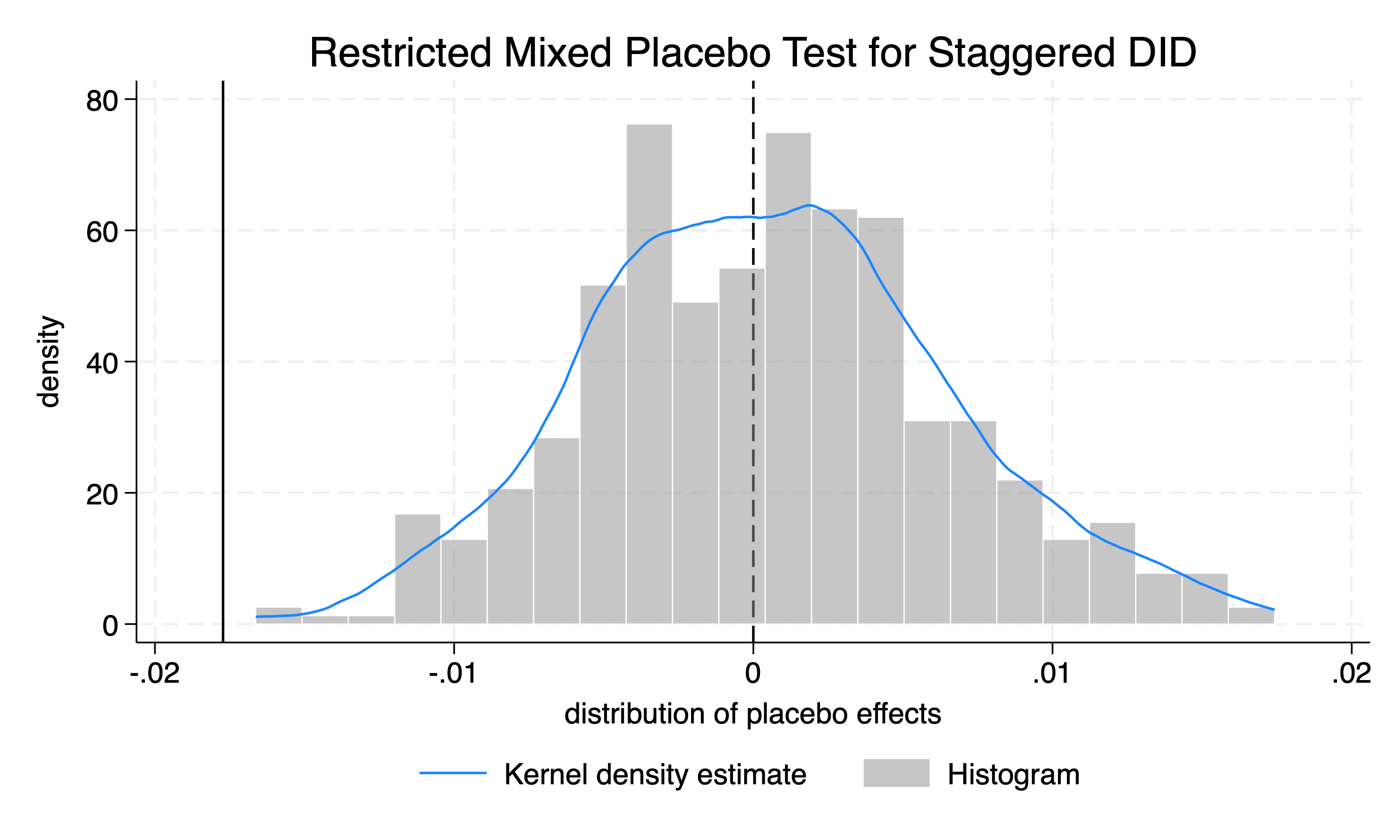
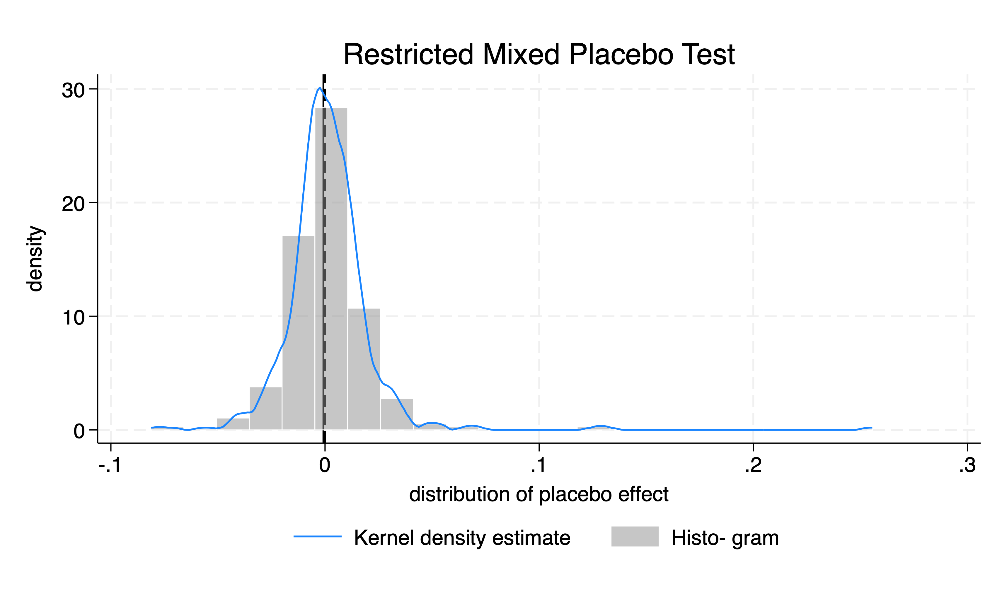
3.3.2 有约束的混合安慰剂检验
指定 pbomix(3) 以进行有约束的混合安慰剂检验,结果展示与交叠 DID 的个体安慰剂检验类似。
Implementing restricted mixed placebo testfor staggered DID (version 3) using both fake treatment units and times: -------------------------------------- The range within which fake treatment times are randomly selected -------------------------------------- [1976, 2000] -------------------------------------- Simulations (500):.........10.........20.........30.........40.........50.........60.........70.........80.........90.........100.........110.........120..... > ....130.........140.........150.........160.........170.........180.........190.........200.........210.........220.........230.........240.........250..... > ....260.........270.........280.........290.........300.........310.........320.........330.........340.........350.........360.........370.........380..... > ....390.........400.........410.........420.........430.........440.........450.........460.........470.........480.........490.........500 Results of restricted mixed placebo testfor staggered DID (version 3) using both fake treatment units and times: -------------------------------------------------------------- | | P-value | Coefficient | Two-sided Left-sided right-sided -----------+-------------+------------------------------------ _intra | -0.017724 | 0.0000 0.0000 1.0000 -------------------------------------------------------------- Note: (1) The two-sided p-value is the frequency that the absolute values of the placebo effects are greater than or equal to the absolute value of estimated treatment effect. (2) The left-sided (right-sided) p-value is the frequency that the placebo effects are smaller (greater) than or equal to the estimated treatment effect.
Finished.
四、基于 csdid 估计的交叠 DID 的安慰剂检验
1. csdid 估计结果
使用 Callaway and Sant’Anna(2021)开发的 csdid 命令,可以实现进行多个干预时点的 DID 估计。csdid 命令基于 drdid 命令开发,并在后续的绘图中需要使用 coefplot 命令,这些都是外部命令,在首次使用前需要进行安装。下面是基于 bbb.dta 数据集使用 csdid 命令进行估计的代码。
. csdid log_gini $cov, ivar(statefip) time(wrkyr) gvar(branch_reform) method(dripw) wboot rseed(1) agg(simple) No never treated observations found. Using Not yet treated data Units always treated found. These will be ignored xxxxxxxxxxxxxxxxxxxxxxxxxxxxxx...........xxxxxxxxx xxxxxxxxxx..........xxxxxxxxxxxxxxxxxxxx...x...... .xxxxxxxxxxxxxxxxxxx..............xxxxxxxxxxxxxxxx .............xxxxxxxxxxxxxxxxx......xxxxxxxxxxxxxx xxxxxxxxxxx.x...x...xxxxxxxxxxxxxxxxxxxx.......... .......xxxxxxxxxxxxx................xxxxxxxxxxxxxx ......................xxxxxxxx.................... ..xxxxxxxxx..xxxx...x...xxxxxxxxxxxxxxxx.......... .......xxxxxxxxxxxxx.x.xx.xxx.xxxx...xxxxxxxxxxxxx xxxxxxxxxxxxxxxxxxxxxxxxxxxxxxxxxxxxxxxxxxxxxxxxxx xxxxxxxxxxxxxxxxxxxxxxxxxxxxxxxxxxxxxxxx Difference-in-difference with Multiple Time Periods
Number of obs = 636 Outcome model : least squares Treatment model: inverse probability --------------------------------------------------------------------- | Coefficient Std. err. t [95% conf. interval] ------------+-------------------------------------------------------- ATT | -.0007548 .0085642 -0.09 -.0174154 .0159058 --------------------------------------------------------------------- Control: Not yet Treated
See Callaway and Sant'Anna (2021) for details
2. 交叠 DID 的时间安慰剂检验
首先,来看看使用基于 csdid 命令估计交叠 DID 的时间安慰剂检验。我们手动生成一个滞后 1 期的干预时间变量,作为伪干预时间用于时间安慰剂检验。使用 if wrkyr < branch_reform 将回归限定在干预前的样本中进行,以进行滞后 1 期的伪干预时间 branch_reform_1 的影响。
. csdid log_gini $covif wrkyr < branch_reform, ivar(statefip) time(wrkyr) gvar(branch_reform_1) wboot rseed(1) agg(simple) No never treated observations found. Using Not yet treated data Units always treated found. These will be ignored Panel is not balanced Will use observations with Pair balanced (observed at t0 and t1) .xxxxxxxxxxxxxxxxxxxxx..xxxxxxxxxxxxxxxxxxxx...xxx xxxxxxxxxxxxxxxx....xxxxxxxxxxxxxxxxxx.....xxxxxxx xxxxxxxxxx......xxxxxxxxxxxxxxxxx.x...xxxxxxxxxxxx xxxx........xxxxxxxxxxxxxx.........xxxxxxxxxxxxx.. ........xxxxxxxxxxxx...........xxxxxxxxxxxx..xxxx. ..x.xxxxxxxxxx.............xxxxxxxxx.x.xx.xxx.xxxx xxxxxxxxxxxxxxxxxxxxxxxxxxxxxxxxxxxxxxxxxxxxxxxxxx xxxxxxxxxxxxxxxxxxxxxxxx Difference-in-difference with Multiple Time Periods
Number of obs = 361 Outcome model : least squares Treatment model: inverse probability --------------------------------------------------------------------- | Coefficient Std. err. t [95% conf. interval] ------------+-------------------------------------------------------- ATT | -.0060173 .0132436 -0.45 -.0333741 .0213396 --------------------------------------------------------------------- Control: Not yet Treated
上面的图片中没有用于判别显著性的 p 值,这里仍然使用 500 次自举法得到 ATT 的 pbo_eff 和真实估计系数 $tr_eff 进行比较,对其进行描述性统计即可得到个体安慰剂的 p 值。具体来看:
双边检验:是否满足 abs(pbo_eff)>=abs($tr_eff),即是否安慰剂检验 ATT 绝对值大于等于真实估计系数绝对值。
左边检验:是否满足 pbo_eff<=$tr_eff),即是否安慰剂检验 ATT 绝对值小于等于真实估计系数绝对值。
右边检验:是否满足 pbo_eff>=$tr_eff),即是否安慰剂检验 ATT 绝对值大于等于真实估计系数绝对值。
其代码实现如下所示:
1 2 3 4 5 6 7 8 9
// 双边检验 g extreme_abs = (abs(pbo_eff)>=abs($tr_eff)) sum extreme_abs // 左边检验 g extreme_left = (pbo_eff<=$tr_eff) sum extreme_left // 右边检验 g extreme_right = (pbo_eff>=$tr_eff) sum extreme_right
上面双边检验、左边检验和右边检验的第一步本质是生成了 500 个虚拟变量(因为自举法重复了 500 次)。双边检验、左边检验和右边检验的均值即为显著性水平 p 值,表明不论在哪一个检验中均不显著,表明 csdid 估计系数和安慰剂效应没有显著区别,安慰剂检验未能通过,上面基准回归的结果并不稳健。
1 2 3 4 5 6 7 8 9 10 11 12 13 14
// 双边检验 Variable | Obs Mean Std. dev. Min Max -------------+--------------------------------------------------------- extreme_abs | 500 .956 .2053005 0 1
// 左边检验 Variable | Obs Mean Std. dev. Min Max -------------+--------------------------------------------------------- extreme_left | 500 .492 .5004367 0 1
// 右边检验 Variable | Obs Mean Std. dev. Min Max -------------+--------------------------------------------------------- extreme_ri~t | 500 .508 .5004367 0 1
// 双边检验 gen extreme_abs = (abs(pbo_eff)>=abs($tr_eff)) sum extreme_abs // 左边检验 gen extreme_left = (pbo_eff<=$tr_eff) sum extreme_left // 右边检验 gen extreme_right = (pbo_eff>=$tr_eff) sum extreme_right
绘图结果如下所示,ATT 的取值位于安慰剂效应分布的中部,并非在极端值位置,估计的ATT(黑色实线)与 0 值(黑色虚线)几乎完全重合,表明 ATT 可能和 0 并无显著差异。
我们进一步看看双边检验、左边检验和右边检验的结果。
1 2 3 4 5 6 7 8 9
// 双边检验 gen extreme_abs = (abs(pbo_eff)>=abs($tr_eff)) sum extreme_abs // 左边检验 gen extreme_left = (pbo_eff<=$tr_eff) sum extreme_left // 右边检验 gen extreme_right = (pbo_eff>=$tr_eff) sum extreme_right
基于比较结果生成的虚拟变量均值,即为混合安慰剂效应双边、左边和右边检验的 p 值。从下面的表中可以发现,三个检验值的均值都超过了 0.1,表明至少在 10% 水平上,未能通过有约束的混合安慰剂检验。
1 2 3 4 5 6 7 8 9 10 11 12 13 14
// 双边检验
    Variable |        Obs        Mean    Std. dev.       Min        Max
-------------+---------------------------------------------------------
 extreme_abs |        500        .966    .1814106          0          1

// 左边检验
    Variable |        Obs        Mean    Std. dev.       Min        Max
-------------+---------------------------------------------------------
extreme_left |        500        .474    .4998236          0          1

// 右边检验
    Variable |        Obs        Mean    Std. dev.       Min        Max
-------------+---------------------------------------------------------
extreme_ri~t |        500        .526    .4998236          0          1
五、写在后面
本文根据陈强等(2025)提供的代码和数据,对标准 DID 和交叠 DID 进行了时间安慰剂、个体安慰剂和混合安慰剂检验。其中交叠 DID 包括有约束和无约束的混合安慰剂检验。针对标准 DID 和使用基于 xtreg 开发的命令(例如 reghdfe)进行交叠 DID 估计的结果,陈强等(2025)开发的 didplacebo 命令可以用于安慰剂检验。对于更加常见的使用 csdid 命令进行交叠 DID 估计的结果,陈强等(2025)也给出了参考的代码用于检验。
当然,DID 系列方法发展迅速,例如放宽样本不允许退出假设的一般 DID、放宽干预行为同质(即存在干预强度差别)的连续 DID、DDD 等方法不断更新,didplacebo 命令不可能服务于所有 DID 类型的安慰剂检验。更加重要的是,参考陈强等对 csdid 命令估计交叠 DID 结果的安慰剂检验思路,设计一个符合自己研究需要的安慰检验代码。

 alipay