
实证|变系数随机前沿分析的简明教程
引用信息:Gong Binlei. Agricultural reforms and production in China: Changes in provincial production function and productivity in 1978–2015[J]. Journal of Development Economics, 2018, 132: 18-31.
在传统的效率分析中,通常使用随机前沿分析(SFA)和数据包络分析(DEA)测算效率。SFA 的生产函数通常设置为 Cobb-Dougles 或者 Translog 形式,并且引入随机误差项来解决外生冲击的影响,例如农业生产中的天气变化。DEA 则不假设生产前沿的具体函数形式,但没有考虑到经济活动具有一定的随机性。
有一些研究对 SFA 和 DEA 进行了改进,尝试解决面板数据中传统效率分析方法的问题,例如 TFE-SFA(True Fixed Effect SFA)、内生 SFA(Endog-SFA)等。然而,这些基于 SFA 方法的改进仍然未解决一个问题:SFA 通常假设投入和产出关系固定不变,其回归系数不能反映随时间变化的投入产出关系。 改革开放以来,我国农业生产关系和生产力水平发生了巨大变化,使用传统的 SFA 方法不能很好反映制度变革和技术变化等带来的农业生产变化。
2018 年,龚斌磊在《 Journal of Development Economics 》上发表《Agricultural reforms and production in China: Changes in provincial production function and productivity in 1978–2015》,提出了一种新的效率分析方法——变系数 SFA(Varying Coefficient SFA) 。变系数 SFA 通过半参数方法,可以估计随时间和个体变化的要素产出弹性和 TFP。
一、变系数 SFA 的简单介绍
1. 适用范围与特点
弹性生产函数。 传统的 SFA 假设生产函数是固定的,无法捕捉随时间变化的投入产出关系。变系数 SFA 允许生产函数的系数随时间变化,能够更好地反映农业生产中随着制度改革、技术进步等因素的变化。
控制外生冲击影响。 与传统 SFA 一样,由于使用 SFA 估计,变系数 SFA 仍然可以通过引入残差项控制外生冲击对投入产出关系的影响,这种估计方程设定更加适合运用在农业的效率分析中。
半参数估计方法。 变系数 SFA 为两步估计,在估计变系数时,需要引入额外的变量来进行半参数估计,这篇文章通过引入各地区农业、林业、牧业、渔业的增加值占比来估计变系数。
2. 分析内容
与传统 SFA 相同,变系数 SFA 可以估计要素产出弹性和技术效率,并进一步计算 TFP 和 TFP 增长率。
简单介绍一下变系数 SFA 的估计方程。
Hastie and Tibshirani (1993) 首先引入了变系数模型(VCM),其中变系数是某些“阈值”变量 \(\theta\) 的非参数函数。
\[ \begin{align} y = x_1 h_1(\theta_1) + \dots + x_p h_p(\theta_p) + \varepsilon \end{align} \]
其中,\(\theta_1, \dots, \theta_p\) 通过未指定函数形式的 \(h_1(\cdot), \dots, h_p(\cdot)\),改变 \(x_1, \dots , x_p\) 系数。
\[ \begin{align} y_{it} & = \alpha_{it} + \sum_{k=1}^{p} \beta_{it}^k x_{it}^k + \tau Z + \nu_{it} - u_i \notag \\\ & = h_0(\theta_{it}) + \sum_{k=1}^{p} h_k(\theta_{it}) x_{it}^k + \tau Z + \nu_{it} - u_i \end{align} \]
其中:
- \(y_{it}\) 表示产出;
- \(x_{it}^k\) 表示第 \(k\) 种投入要素;
- \(h_k(\theta_{it})\) 表示非参数函数,用于估计第 \(k\) 种投入要素的变弹性 \(\beta_{it}^k\)。
二、变系数 SFA 的简明教程
我们重点关注怎么使用变系数 SFA 方法。
1. 基础处理
基础处理包括:(1)导入相关 R 包;(2)简单处理数据。
1 | library('gss') |
2. 传统 SFA
控制时间固定效应的传统 SFA,技术无效效率项服从截断正态分布(truncated normal distribution)。
1 | single <- sfa(Y~Lr+Ld+Fr+Kp+Year, timeEffect=TRUE, truncNorm=TRUE, data=pdata) |
3. 变系数 SFA
变系数 SFA 的第一步是要进行半参数估计,得到 \(h_k(\theta_{it})\),这一步使用 GAMLSS 模型进行估计。第二步是基于 GAMLSS 模型的结果,计算变系数、残差、效率值等。需要使用 Bootstrap 法逐年估计置信区间,用于绘图使用。
1 | # 定义模型:使用 Generalized Additive Models for Location, Scale and Shape (GAMLSS) 拟合模型 |
三、结果分析
上述代码已经完成变系数 SFA 的估计,但是由于模型为每个样本、每个要素都计算了一个系数,无法通过表格的方式展示所有回归系数,需要通过绘图的方式进行展示。
1. 年度要素弹性比较
该部分绘制了劳动、土地、化肥和机械四种要素的产出弹性年度变化图。
1 | # Figure 2 Average Elasticities of the Four Inputs across Time |
结果展示:

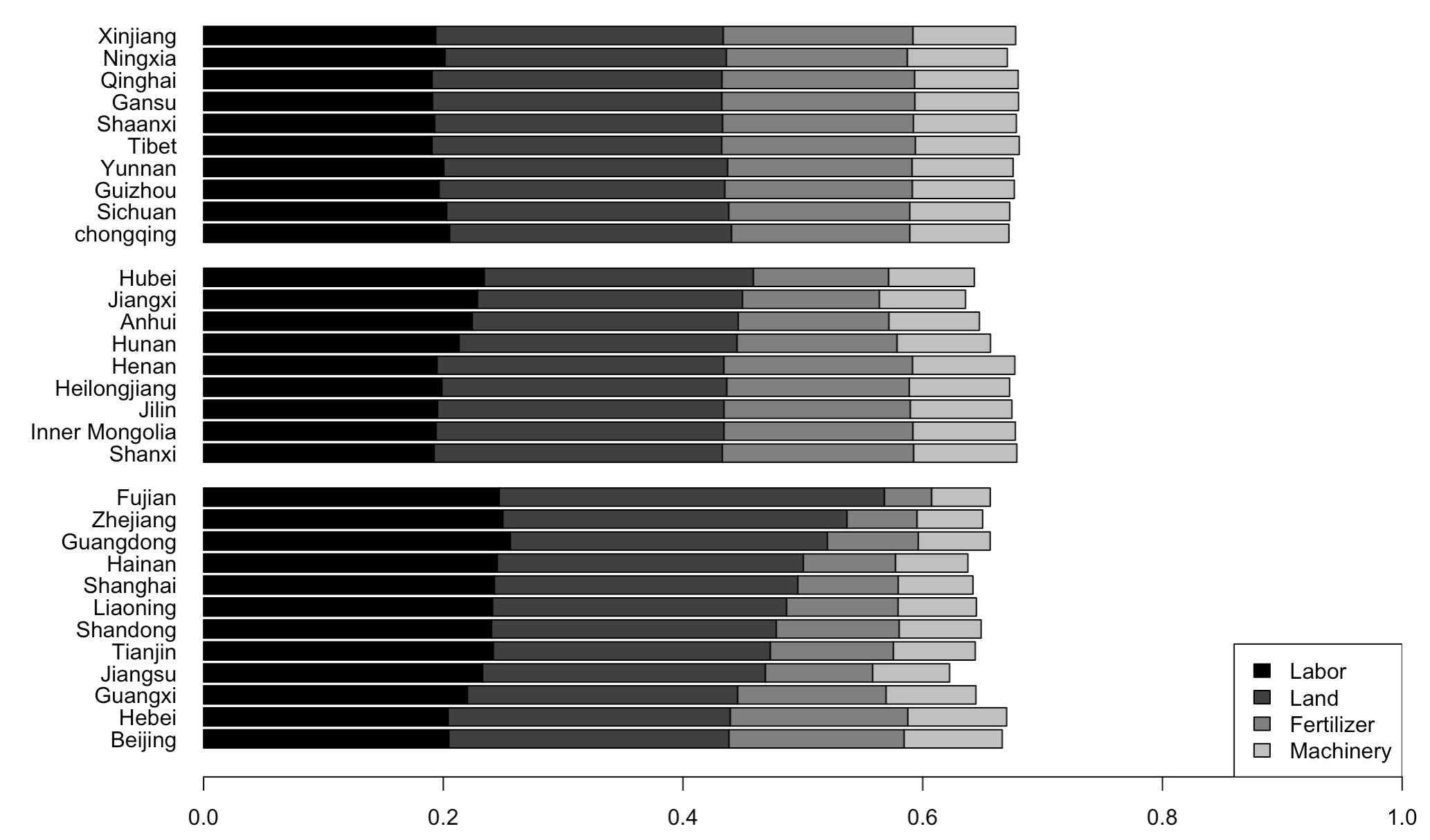
2. 省际要素弹性比较
在完成年度比较后,可以从个体的维度(省份)去考察区域间要素产出弹性差异。
1 | # Figure 3 Average Elasticities of the Four Inputs across Provinces |
图片展示:
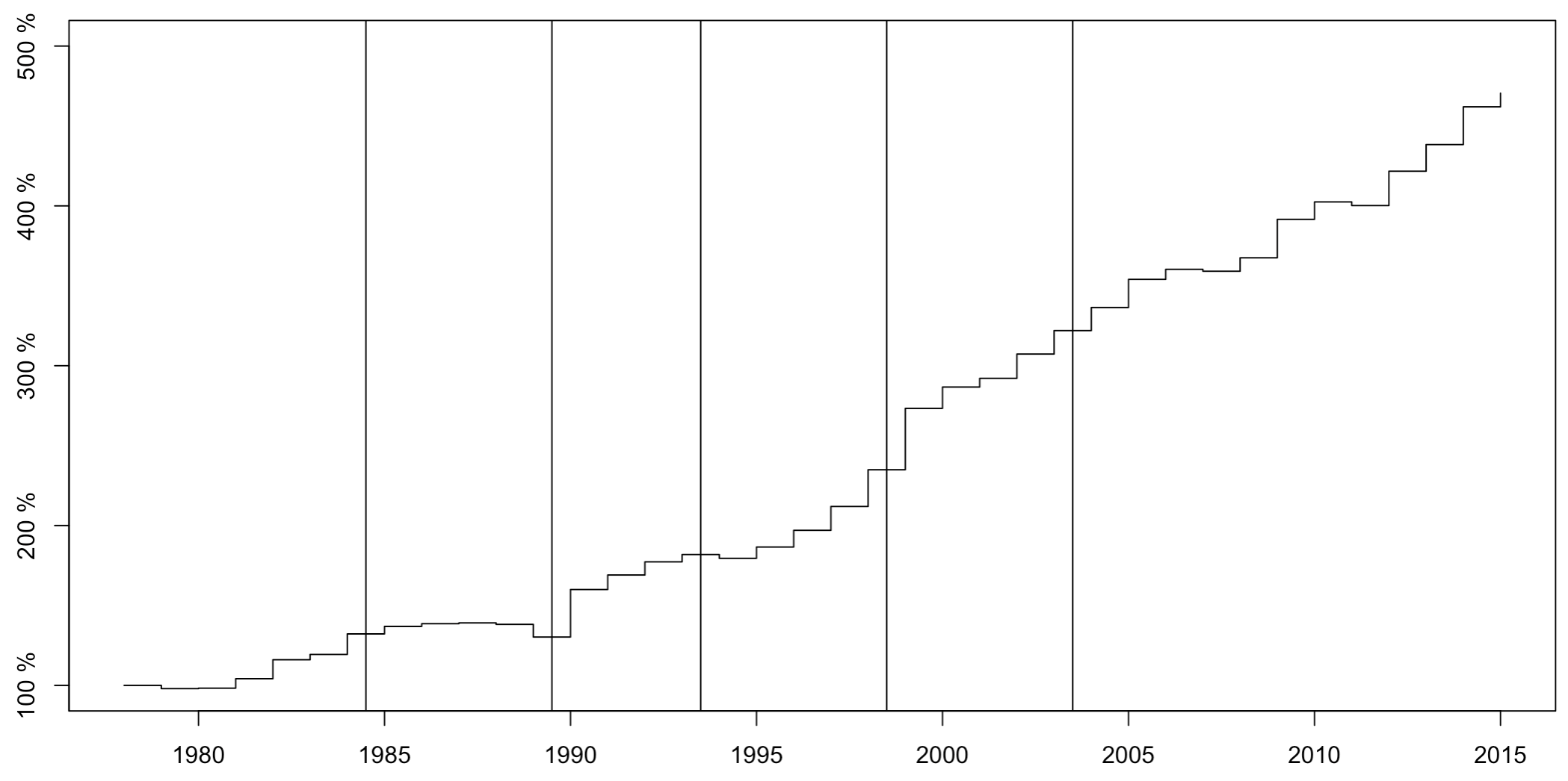
3. 年度技术变化分析
上面两个部分都是针对要素产出弹性的分析,下面是对技术变化的年度分析。这里需要根据上面的结果,进一步计算技术变化指标。
1 | # Technology Growth |
图片展示:
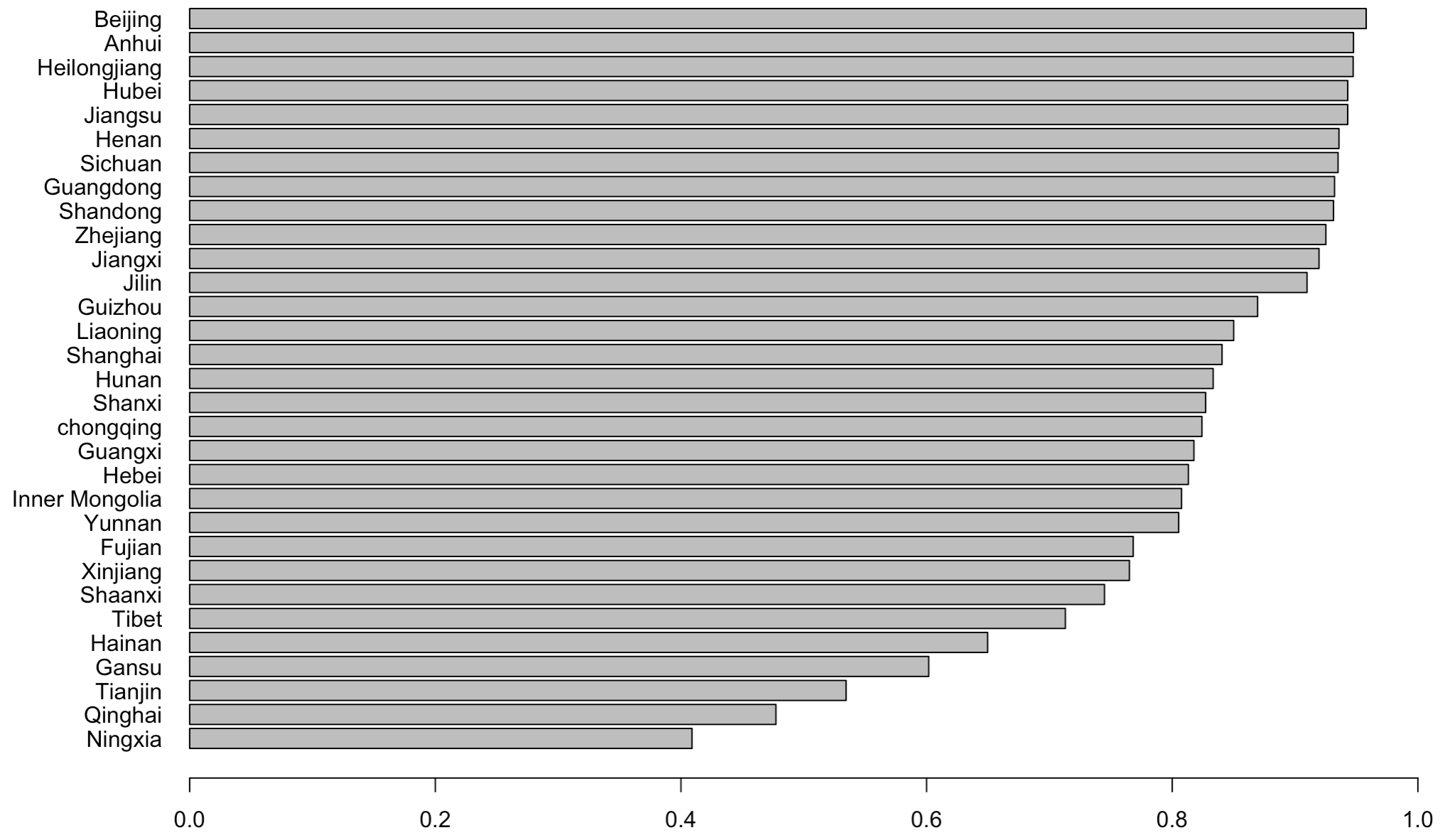
4. 省际技术效率比较
再来考察一下技术效率。
1 | # Efficency |
图片展示:
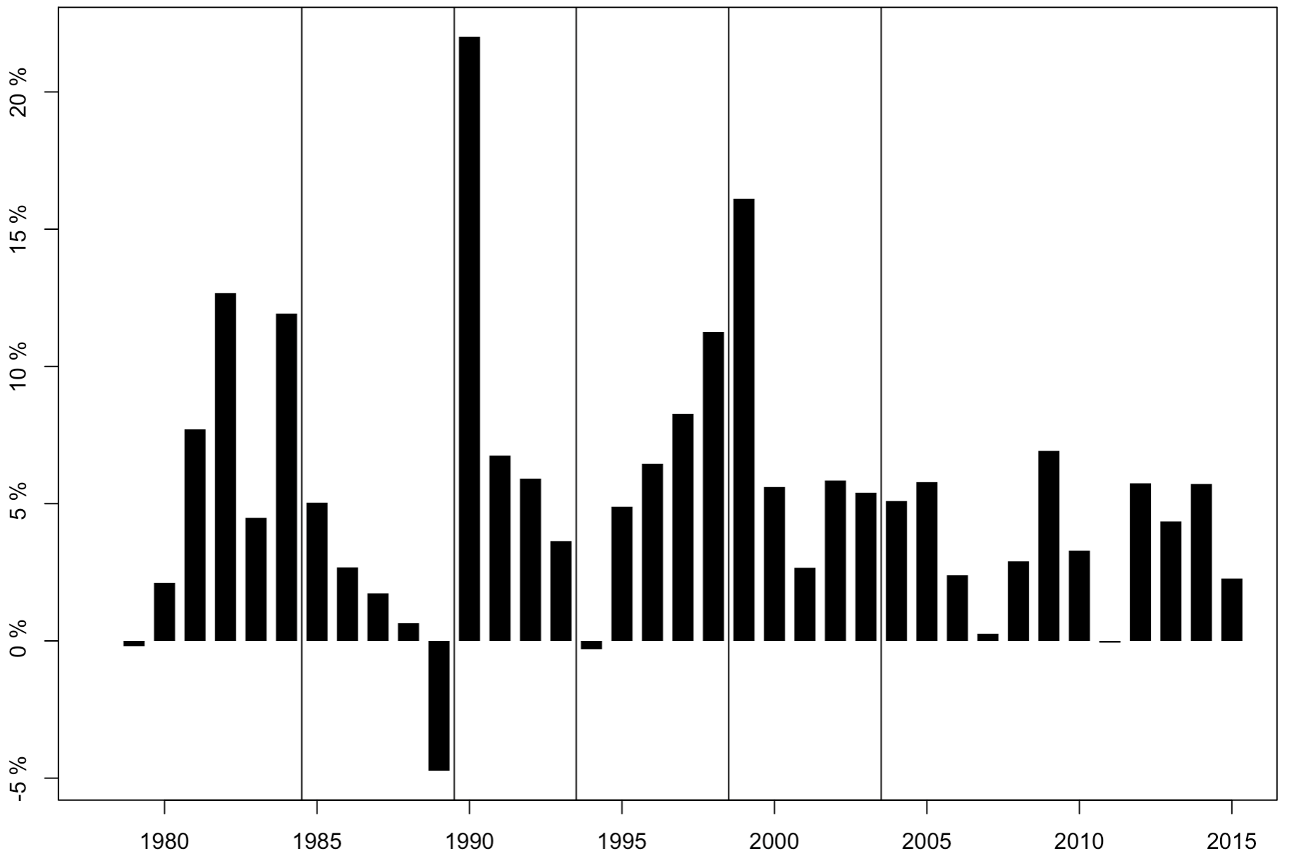
5. TFP 增长率变化
再来看看 TFP 增长率的年度变化。
1 | # TFP |
图片展示:
四、写在后面
变系数 SFA 法是解决传统 SFA 固定投入产出关系问题的一大利器,不过该方法仍然有一些小问题。一是该方法针对省级面板数据开发,且计算过程涉及矩阵运算,要求数据为平衡面板, 非平衡面板数据可能中间部分代码会报错。二是变系数 SFA 的要素产出弹性和 TFP 估计受到第一步半参数估计的影响,导致部分样本差异化的系数估计结果难以解释, 针对这一问题,应重点关注变系数 SFA 是否正确运用,同时注意检验结果的可靠性。
在这篇文章的后半部分,还基于上面的结果进行了实证分析。这里不在赘述,有兴趣可以查看原文。
下面附上文章 PDF、完整代码和数据,可用于代码复现。官方的代码有一些小 bug,且没有代码备注,检验使用「Code and Data (JDE)」文件夹内的代码复现。
下载链接:百度网盘链接
 alipay